import matplotlib
import matplotlib.pyplot as plt
from matplotlib import rc, font_manager
matplotlib.pyplot객체를 plt로 정의하고 불러옴
맷플랏립에서 font_manager와 rc를 불러옴
근데 여기있는 예시는 mac에선 안 돌아감. 디렉도리가 윈도우라 알아서 찾아보삼
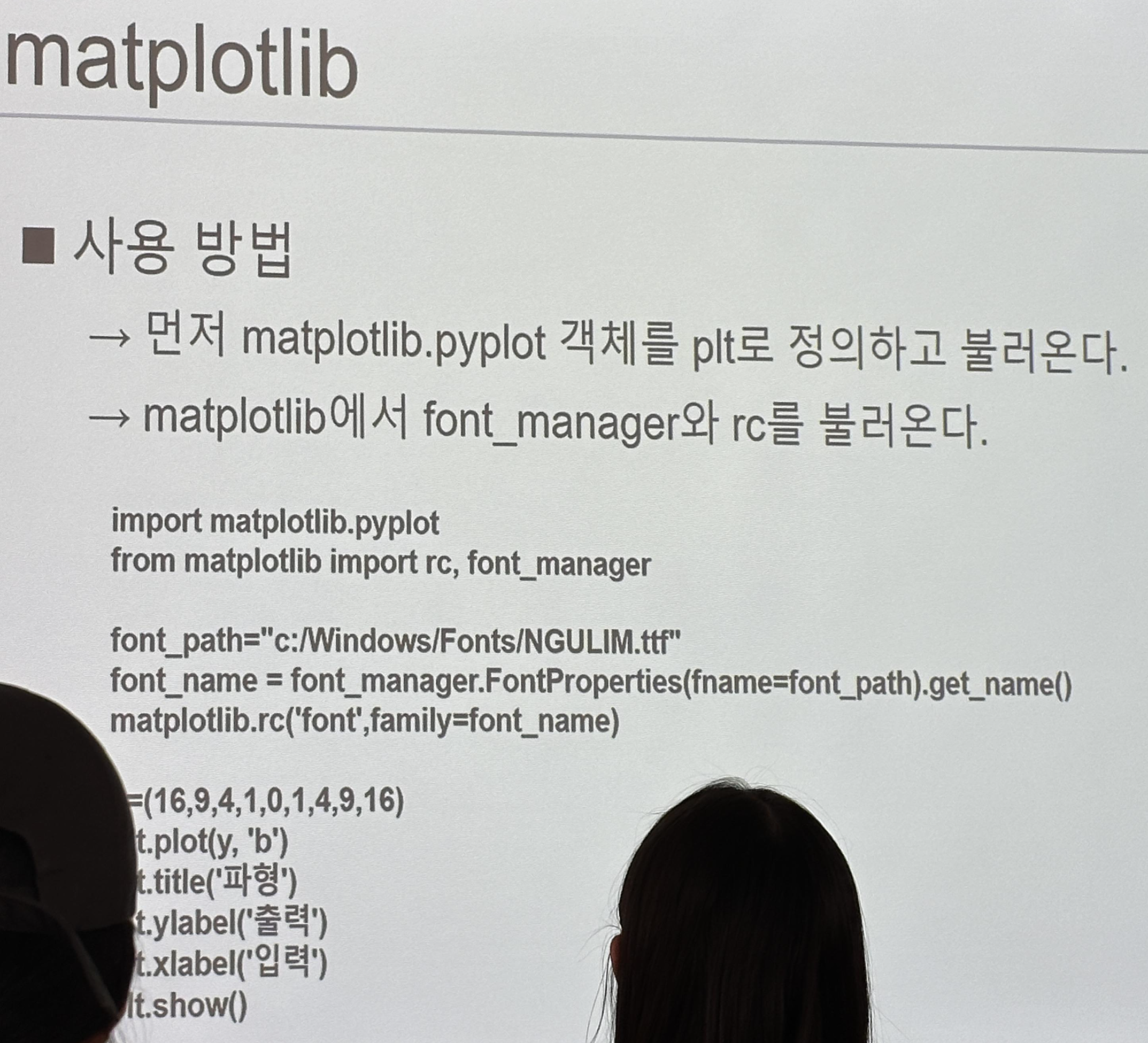
import matplotlib.pyplot as plt
from matplotlib import rc, font_manager

#font_path="c:/Windows/Fonts/NGULIM.ttf" #이부분은 맥에 맞게 조정 필요. 안 돌아감 그 전까진
#font_name = font_manager.FontProperties(fname=font_path).get_name()
#rc('font',family=font_name)
x = list(range(-10,11,1))
y= [i**2 for i in x]#원래 와이 y=(16,9,4,1,0,1,4,9,16)
plt.plot(x,y, 'b')
plt.title('Signal')
plt.ylabel('Output')
plt.xlabel('Input')
plt.show()


import matplotlib.pyplot as plt
plt.plot([1,3,7,11,14,15 ]) # distance
plt.xlabel('time[min]')
plt.ylabel('distance[km]')
plt.show()


plt.plot([1,2,3,4,5],[120,200,160,350,110])
plt.xlabel('input')
plt.ylabel('output')
plt.title('Experiment Result')
plt.show()
#항상 0부터 시작할 필요 없고 - 들어갈 필요 없음 알아서 정하면 됨.

#조금 더 강조하고 포인트를 주고싶다.?
#r red s square -- 점선// rs--, sr--이것도 동일.
라이브러리 폴더 지정 해주기 . 윈도우 버전이라 안됨. ㅜㅜ
import matplotlib.pyplot as plt
plt.title("plot subject", loc='center', fontdict={'fontsize': 14}) # title
plt.plot([10, 20, 30, 40], [1, 4, 9, 16], 'c*--')
plt.xlabel("time", fontdict={'fontsize': 14}) # x-axis label
plt.ylabel("amplitude", fontdict={'fontsize': 14}) # y-axis label
plt.xlim(0, 50)
plt.ylim(0, 20)
plt.show()- rs-- 이런 느낌으로 포인트 줄 수 있음. 궁금하면 matplotlib 검색해서 색상 모양정보 알아보자
- 색 두개 지정은 안됨.
- 폰트사이즈 지정 가능.
- loc는 로케이션. center이면 가운데임 ㅇㅇ
- x,y limit 정해주지 않으면 적당히 사각형 안쪽 범위로만 지정해줌. 구체적 범위 지정하고 싶다면 lim값 지정 필요.
import matplotlib.pyplot as plt
x = range(0, 5)
y = [v**2 for v in x]
s = [1000, 200, 300, 400, 500]
plt.scatter(x = x, y = y, s = s, c = 'red', alpha=0.9)
plt.show()


from matplotlib import pyplot as plt
plt.plot([1,2,3,4], [1,4,9,10], 'rs--')
plt.plot([2,3,4,5],[5,6,7,9], 'b^-')
plt.xlabel('input')
plt.ylabel('output)')
plt.title('Experiment Result')
plt.legend(['Dog', 'Cat'], loc='lower right')
plt.show()- scatter plot 표현 가능
- alpha는 투명도를 표현.
- 그래프 두개를 하고 싶다면 plt.plot을 두개 지정해 주면 됨.
import matplotlib.pyplot as plt
x = range(0, 100)
y1 = [v**2 for v in x]
y2 = [v**3 for v in x]
plt.subplot(2, 1, 1)
plt.ylabel('v^2')
plt.plot(x, y1)
plt.subplot(2, 1, 2)
plt.ylabel('v^3')
plt.plot(x, y2)
plt.grid()
plt.show()- 격자 만들어 주고 싶다면 grid 이용
- subplot - 행과 열 인자로 받고 맨 뒤에 plot 순서 지정. plt.subplot(2,1,1) 이런 느낌.
- subplot 지워버리면
이런 모양이 나옴
- figure - figsize 이용하면 그래프 전체 비율 조정 가능
from matplotlib import pyplot as plt
import numpy as np
x = range(0, 20)
y = [v**2 for v in x]
plt.bar(x, y, width=0.5, color="red")
plt.show()

# tick locations and labels
plt.xticks(np.arange(6),('xtick1', 'xtick2', 'xtick3','xtick4', 'xtick5', 'xtick6'))

plt.yticks([0,5,10,15,20,25], ('ytick1', 'ytick2', 'ytick3','ytick4', 'ytick5', 'ytick6'))

# ticks, tick labels, and gridlines
plt.tick_params(axis='x', labelsize=13, colors='b')
plt.tick_params(axis='y', labelsize=13, colors='r')
plt.grid()
plt.show()- 인덱스 텍스트별로 출력.. 중요하대요!!! / 저 xtick ytick이 인덱스별 텍스트 입력임 ㅇㅇ. // 이거꼭 기억하삼. 교수님이 강조하심
import matplotlib.pyplot as plt
import numpy as np
plt.figure(figsize=(10,2))
x = np.linspace(0, 1.0)
y = np.cos(np.pi*2*x)**2
plt.plot(x, y)
plt.show()

plt.figure(figsize=(10,2))
x = np.linspace(0, 1.0)
y = np.cos(np.pi*2*x)**2
plt.plot(x, y, marker='x', markersize=8, linestyle=':', linewidth=3,
color='g', label='$\cos^2(\pi x)$')
plt.legend(loc='lower right')
plt.xlabel('input')
plt.ylabel('output')
plt.title('Experiment Result')
plt.show()

import matplotlib.pyplot as plt
import numpy as np
plt.figure(figsize=(10,2))

plt.figure(figsize=(10,2))
x = np.linspace(0, 1.0)
y = np.cos(np.pi*2*x)**2
plt.plot(x, y, marker='x', markersize=8, linestyle=':', linewidth=3,
color='g', label='$\sin^2(\pi x)$')
plt.legend(loc='lower right')
plt.xlabel('input')
plt.ylabel('output')
plt.title('Experiment Result')
plt.savefig('func_plot.jpg')
plt.show()

import matplotlib.pyplot as plt
fig = plt.figure(figsize=(10, 4))
for subplot in range(1, 7):
    axis = fig.add_subplot(2, 3, subplot)
fig.tight_layout();
plt.show()
fig = plt.figure(figsize=(10, 3))
t = np.linspace(0.0, 1.0)
for subplot in range(1, 7):
    axis = fig.add_subplot(2, 3, subplot)
    axis.plot(t, np.cos(2*np.pi*t*subplot)+1)
    axis.set_xlabel('time[s]')
    axis.set_ylabel('voltage[mV]')
    axis.set_title('$\cos({} \pi t)$ +1'.format(subplot))
fig.tight_layout()
plt.show()


import matplotlib.pyplot as plt
from mpl_toolkits.mplot3d.axes3d import Axes3D
fig = plt.figure(figsize=(10, 5))
axis = fig.add_axes([0.1, 0.1, 0.8, 0.8], projection='3d')

import numpy as np
t = np.linspace(0.0, 5.0, 500)
x = np.cos(np.pi*t)
y = np.sin(np.pi*t)
z = 2*t
axis.plot(x, y, z)
axis.set_xlabel('x-axis')
axis.set_ylabel('y-axis')
axis.set_zlabel('z-axis')
plt.show()- savefig하면 지정한 이름대로 그래프 파일이 새로 생김
- tight_layout() 하면 ... 응애 뭐 어케되는데
- 3차원도 만ㄷ르 수 잇음. 근데 성능 안 좋으면 컴터 멈출지도 ㄷㄷ
import matplotlib.pyplot as plt
from mpl_toolkits.mplot3d.axes3d import Axes3D
fig = plt.figure(figsize=(10, 5))
axis = fig.add_axes([0.1, 0.1, 0.8, 0.8], projection='3d')
x = np.linspace(0.0, 1.0) # x, y are vectors
y = np.linspace(0.0, 1.0)
X, Y = np.meshgrid(x, y) # X, Y are 2d arrays
Z = X**2 -Y**2 # points in the z axis
axis.plot_surface(X, Y, Z) # data values (2D Arryas)
axis.set_xlabel('x-axis')
axis.set_ylabel('y-axis')
axis.set_zlabel('z-axis')
axis.view_init(elev=30,azim=70) # elevation & angle
axis.dist=10 # distance from the plot
plt.show()

from matplotlib import cm
fig = plt.figure(figsize=(10, 5))
axis = fig.add_axes([0.1, 0.1, 0.8, 0.8], projection='3d')
p = axis.plot_surface(X, Y, Z, rstride=1, cstride=2, cmap=cm.coolwarm,
linewidth=1)
axis.set_xlabel('x-axis')
axis.set_ylabel('y-axis')
axis.set_zlabel('z-axis')
axis.view_init(elev=30,azim=70) # elevation & angle
fig.colorbar(p, shrink=0.5);
plt.show()- surface 방식으로 3차원 만들 수 있음. 개신기하넼ㅋ // top에서 보면 높이 분간이 불가함.
- 이 문제점을 고치기 위해 컬러바를 작성해서 높이를 알아보기 쉽게 함. 근데 3D문제는 안 나올 듯
<시험!!!!!!!!>
- 시험은 기본 선형 그래프와 scatter, subplot, bar형태. xtick, ytick 등 중점적으로 연습하면 좋을 듯 // xtick 별도로 ytick별도로 연습하면 조금 더 도움이 됨.
- scipy시험범위에 들어감
'Pworkspace' 카테고리의 다른 글
| week12 - pandas (11주차에 조금 당겨서 배움) (0) | 2024.05.17 |
|---|---|
| week11 - numpy(2)(histogram+ 너구리) (0) | 2024.05.14 |
| week7 + 중간고사 공지 (0) | 2024.04.16 |
| week3 - split, map , sep, end (0) | 2024.04.05 |
| week3 - format (0) | 2024.04.05 |